

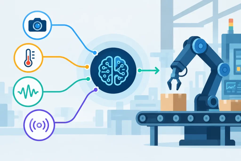
A bearing fault rarely announces itself in one channel. Vibration may show a developing frequency component, acoustic data may capture intermittent impacts, temperature may remain normal, and machine vision may reveal no visible symptom at all. The top sensor fusion techniques address this gap by combining evidence across sensors without forcing every industrial application into an oversized AI architecture.
For industrial automation teams, fusion is not simply a data-science exercise. It is an engineering decision that affects latency, controller resources, fault tolerance, model maintenance, and how easily a system can be validated on the production floor. The right approach depends on whether the system must classify a signal in milliseconds, estimate a physical state continuously, or trigger a reliable machine action from incomplete data.
What Sensor Fusion Must Solve in Industrial Systems
A fusion system combines measurements that differ in sampling rate, units, noise profile, placement, and reliability. A camera can produce frames at 30 fps, an accelerometer may sample at tens of kilohertz, and a programmable logic controller may expose process variables only every 100 milliseconds. Combining those streams without a time reference can create false correlations that look convincing in a test set and fail under live operating conditions.
The first requirement is synchronization. Each input needs a trustworthy timestamp, a known acquisition delay, and a defined resampling strategy. For rotating machinery, alignment should also account for shaft speed and cycle position. A vibration window captured before a load change should not be fused with motor current recorded after it.
The second requirement is sensor confidence. Sensors drift, cables fail, lenses become contaminated, and microphones respond to changes in ambient noise. A useful fusion design does not treat every measurement as equally credible. It monitors signal quality and allows a degraded channel to receive less influence or be excluded while the system continues operating safely.
Finally, fusion must match the action being requested. A system that stops a press, diverts a defective part, or alarms on a safety-relevant condition needs explainable confidence thresholds and conservative fallback behavior. A system that prioritizes maintenance inspections can accept more uncertainty if it reduces missed early-stage faults.
Top Sensor Fusion Techniques by Integration Level
The most practical way to compare top sensor fusion techniques is by the point at which data streams are combined. This choice establishes the computational load, data bandwidth, and diagnostic traceability of the final system.
Early Fusion: Combine Raw or Aligned Measurements
Early fusion combines measurements before substantial feature extraction. For example, an application may align vibration, motor current, speed, and process load data into one multichannel time window. A model then learns relationships across the original or lightly processed signals.
This method can preserve information that later processing might discard. It is useful when the interaction between channels is itself diagnostic, such as the relationship between acoustic impulses and motor current variation during a specific phase of a machine cycle. It can also support multichannel neural models when sufficient representative training data is available.
Its cost is substantial. Raw data streams require high bandwidth, consistent timing, substantial memory, and careful normalization. Adding a sensor can require retraining the complete model. Early fusion is therefore best suited to tightly integrated sensing systems with controlled acquisition hardware and a clear benefit from cross-signal detail.
Feature-Level Fusion: Combine Engineered or Learned Features
Feature-level fusion processes each sensor stream independently before combining compact descriptors. A vibration channel may contribute spectral energy, kurtosis, envelope features, and order-related peaks. An image stream may contribute defect geometry, texture statistics, or neural embeddings. Temperature, pressure, and controller values may enter as normalized scalar features.
For many industrial applications, this is the most balanced architecture. Feature extraction removes unnecessary data volume while preserving diagnostic indicators that engineers can inspect. It also allows each modality to use an appropriate processing method rather than forcing video, audio, and accelerometer data into a single raw-data representation.
Feature-level fusion works well on embedded platforms because the final classifier receives a small, structured feature vector. It also supports staged deployment: a maintenance team can begin with vibration and process features, then add acoustic or visual features when the operational value is proven. The limitation is that poor feature selection can hide interactions that a raw-data model might have learned.
Decision-Level Fusion: Combine Independent Classifiers
Decision-level fusion combines outputs from separate models rather than their input data or features. A vision model may classify surface condition, an acoustic model may classify impact events, and a vibration model may estimate bearing condition. A fusion layer then combines their labels, confidence scores, or anomaly levels.
This approach is particularly effective when sensors are installed on separate subsystems or have incompatible timing. Each recognition path can be tested, calibrated, and maintained independently. It also offers clear diagnostic reporting: operators can see which channel produced an alert and whether another channel confirmed it.
Decision fusion is often implemented through weighted voting, rule logic, confidence thresholds, or probabilistic combination. It is not automatically less capable than early fusion. When the source models are well designed and sensor failures are common operational concerns, independent classifiers can produce a more maintainable system than one large multimodal model.
Estimation Methods for Continuous State Tracking
Classification fusion answers questions such as whether a defect pattern is present. State-estimation fusion answers a different question: what is the most likely current condition of a moving or changing process?
Kalman and Extended Kalman Filtering
Kalman filtering combines a predicted system state with noisy measurements. In industrial equipment, the predicted state may represent position, velocity, temperature, orientation, or another continuously changing variable. The filter adjusts its estimate as new sensor readings arrive, weighted by their expected uncertainty.
A standard Kalman filter is appropriate when the process and measurement relationships are approximately linear. An Extended Kalman Filter linearizes nonlinear relationships around the current estimate, making it useful for applications such as mobile equipment positioning, robotic motion, or nonlinear process models.
These methods are computationally efficient and provide a disciplined way to handle noisy sensors. Their weakness is model dependence. If the physical model or noise assumptions are inaccurate, the estimate can become biased. They are best used where system behavior is known well enough to define a meaningful prediction model.
Particle Filters and Nonlinear Probabilistic Methods
Particle filters represent several possible states rather than a single Gaussian estimate. They can track nonlinear behavior and multiple competing explanations, such as equipment operating in one of several modes. This is valuable when measurements are ambiguous or process dynamics change abruptly.
The trade-off is computational cost. A particle filter may require many particles to maintain accuracy, which can be difficult on constrained embedded hardware. It is justified where ambiguity is central to the application, not simply because the method is mathematically flexible.
Bayesian Evidence and Dempster-Shafer Fusion
Bayesian fusion combines probabilities using prior knowledge and observed evidence. It can incorporate operating context directly: a vibration pattern may have a different meaning at high load than at idle speed. This makes Bayesian approaches useful for condition monitoring systems that must interpret signals within a known process state.
Dempster-Shafer theory is useful when a system needs to distinguish uncertainty from disagreement. A camera may provide little usable evidence because of poor illumination, while an accelerometer may actively indicate a conflicting condition. Those are different situations, and evidence-based fusion can preserve that distinction.
Both approaches require disciplined confidence calibration. A classifier score is not automatically a probability. If confidence values are poorly calibrated, a fusion layer can amplify false certainty instead of reducing it.
Learned Fusion Models and Their Limits
Neural fusion models can learn cross-modal relationships that are difficult to express through fixed rules. Architectures may combine separate sensor encoders with a shared fusion layer, use attention mechanisms to emphasize informative channels, or process time sequences through recurrent or temporal convolutional layers.
This is valuable when fault signatures emerge only from combined patterns, such as a visual variation that matters only when paired with a specific acoustic event. However, learned fusion needs representative data across operating modes, material variations, environmental conditions, and known sensor degradation states. A model trained on synchronized laboratory data may perform poorly when deployed with real communication jitter and maintenance-related changes.
For edge deployment, the architecture should be proportionate to the decision. A compact per-sensor recognizer followed by feature or decision fusion can provide lower latency and easier fault isolation than a centralized deep network. Trainable neural controllers can be especially effective where recognition must remain close to the machine and where cloud connectivity is not appropriate for the control loop. NeuroTechnologijos hardware architectures support this edge-oriented pattern by pairing trainable recognition with deployment formats suited to embedded and industrial integration.
Selecting a Fusion Architecture for the Machine
Start with the failure mode, not the available sensor inventory. If a defect is visible but acoustically silent, vision should lead and other channels should provide context. If the earliest evidence appears in high-frequency vibration, a camera should not be treated as an equal source merely because one is available.
Then define the required response time. Fast rejection or machine protection often favors local feature extraction and decision-level fusion. Process optimization or maintenance analysis can tolerate longer windows and more complex probabilistic estimation. Also define what happens when a channel becomes unavailable. A fusion system should specify whether it continues at reduced confidence, requests inspection, or transitions to a safe state.
Validation must include normal production variation, not only labeled fault samples. Test sensor dropout, delayed data, shifted load profiles, lighting changes, and communication interruptions. Measure false alarms and missed detections by operating condition, because an average accuracy figure does not describe the cost of an error on a live machine.
The most effective fusion system is usually the one that gives each sensor a specific job, preserves timing and confidence information, and produces an action that operators can trust. Start with an architecture that can be verified on the machine, then add complexity only when the additional sensor relationship changes the quality or speed of the decision.
